
While one would think higher interest rates and a reduced balance sheet both currently being employed by the Fed, would hamper inflation, there exists a well-known financial identity that argues otherwise.
In this article, we closely examine the Monetary Exchange Equation with a focus on monetary velocity. Decomposing this simple formula and extracting the inflation identity shows precisely how the level of economic activity and the Fed’s monetary actions come together to affect price levels. This analysis demonstrates that the broadly held and seemingly logical conclusions are incorrect.
Might it be possible the Fed is stoking the embers of inflation while the world thinks they are being extinguished?
Monetary Exchange Equation
To understand how the Fed’s commitment to continued interest rate hikes and balance sheet reduction (Quantitative Tightening –QT) affect inflation or deflation,the Monetary Exchange Equation should be analyzed closely.The equation is not a theory, like most economic frameworks based on assumptions and probabilities. The equation is a mathematical identity, meaning the result will always be true no matter the values of its variables.The monetary exchange equation is as follows:
PQ = MV
The equation states that the amount of nominal output purchased during any period is equal to the money spent. Said differently, the price level (P) times real output (Q) is equal to the monetary base(M) times the rate of turnover or velocityof the monetary base(V).The monetary base-currency plus bank reserves, is the only part of the equation that the Federal Reserve can directly control.Therefore, we believe to form future price expectations, an analysis of the Monetary Exchange Equation using the forecasted monetary base is imperative.
The Inflation Identity
Through simple algebra, we can alter the Monetary Exchange Equationand solve for prices. Once the formula is rearranged, the change in prices (%P) can be solved for, as shown below. In doing so, what is left is called the Inflation Identity.
%P = %M + %V - %Q
Before moving on, we urge you to study the equation above. The logic of this seemingly modest formula is often misunderstood. It is not until one contemplates how M, V,and Q interact with each other to derive price changes that the power of the formula is fully appreciated.
Per the inflation identity, the rate of inflation or deflation (%P) is equal to the rate of money growth (%M), plus the change in velocity (%V), less the rate of output growth (%Q).The word “less” is highlighted because in isolation, assuming no changes in the monetary factors(%M and %V), inflation and economic growth should have a near perfect negative relationship. In other words, stronger economic growth leads to lower prices and vice versa. While that relationship may seem contradictory, consider that more output increases the supply of goods, therefore all other things being equal, prices should decline. Alternatively, less output results in less supply and higher prices.
It is important to note that the inflation identity solves for the GDP deflator, which is one of the price indices on which the Fed relies heavily. While the equation does not solve for the more popular consumer price index (CPI), the deflator is highly correlated with it. The graph below highlights the perfect (correlation = 1.00) relationship between the deflator and the price identity as well as the durable, but not perfect (correlation = 0.93), relationship of CPI to the deflator and price identity.
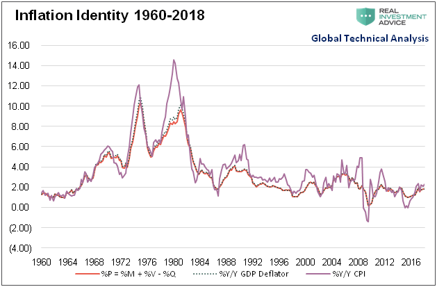
Data Courtesy: Federal Reserve
Let us now discuss %M, %V and %Q so we can consider how %P may change in the current environment.
%M –As noted earlier, the change in the monetary base is a direct function of the Fed’s monetary policy actions. To increase or decrease the monetary base the Fed buys and sells securities, typically U.S. Treasuries and more recently Mortgage-Backed Securities (MBS). For example, when they want to increase the money supply, they create (print) money and distribute it via the purchase of securities in the financial markets. Conversely, to reduce the monetary base they sell securities, pulling money back out of the system. The Fed does not set the Fed Funds rate by decree. To target a certain interest rate they use open market transactions to increase or decrease money available in the Fed Funds market.
Beginning in 2008 with Fed Funds already lowered to the zero bound, the Fed, aiming to further increase the money supply, resorted to Quantitative Easing (QE). Through QE, the Fed bought large amounts of Treasuries and MBS from primary dealers on Wall Street. Largely through this action, the monetary base increased from $850 billion to $4.13 trillion between 2008 and 2015.
%V –Velocity is calculated as nominal GDP divided by the monetary base (Q/M). Velocity measures people's willingness to hold cash or how often cash turns over. Lower velocity means that people are hoarding cash, which usually happens during periods of economic weakness, credit stress, and fear for the going-concern of banking institutions. In contrast, higher velocity tends to result in people avoiding holding cash. This typically happens during times of economic growth, lack of credit stress, and rising interest rates. During such periods, the opportunity cost of physically holding cash increases, as cash holders are incentivized by rising interest rates on deposits and/or productive returns on money in other investments.
Unlike the monetary base, velocity is influenced by the Fed through interest rates butnot directly controlled by the Fed. The graph below shows the relationship between the Fed Funds effective rate and velocity.
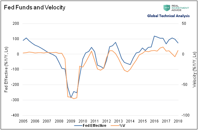
Data Courtesy: Federal Reserve
The deflation of the Great Depression occurred as credit stress, weak economic growth, and bank failures created an acute demand by the public to hold money. It was deemed safer to stuff your mattress with cash than to trust a bank to hold it for you. The effect was a sharp decline in velocity (%V). When coupled with inadequate growth in the monetary base (%M), the combination overwhelmed the inflationary impact of lower output growth (%Q). The result of this effect was deflation (%P).
Similar to the Great Depression, velocity dropped precipitously during and coming out of the Great Financial Crisis of 2008.Determined not to make the same perceived mistake, the Fed under Ben Bernanke increased the monetary base substantially. After cutting Fed Funds to zero and executingthree rounds of QE, its balance sheet increased from $800 billion to over $4 trillion as shown below.Partially as a result of these actions,theGDP Deflator never registered a negative year-over-year reading but, and this point is critical, neither did it spike higher as was forecast by critics of QE.
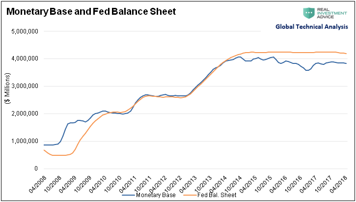
Data Courtesy: Federal Reserve
%Q – Like velocity,the level of economic output (Q) is not directly set by the Fed,but it is influenced by their actions. The supply and demand for credit, and therefore related economic activity, ebbs and flows in part based on the Fed’s interest rate policy.Historically the Fed will raise rates when economic growth “runs hot,” and inflationary pressures are on the rise. Alternatively, the Fed lowers rates to spur economic activity, incentivize borrowing, and boost inflation (or avoid deflation) when economic conditions are weak or recessionary.
The Fed’s influence on output (Q)varies over time as it is heavily dependent on the composition of economic growth. Currently, with demographics and productivity providing little support for economic growth, debt (be it government, corporate or household) has been a predominant driver of economic activity. In such an environment, one can presume that the level of interest rates plays a bigger role in determining output (%Q) than one in which debt is not the primary driver of growth. This factor helps explain why double-digit interest rates in the 1970’s, although painful, did not crush economic growth yet investors today are fretting over a 3.0% yield on Ten-Year Treasury Notes.
Current Monetary Dynamics
Since 2015 the Fed has increased the Fed Funds rate six times, bringing it from the range of 0.00-0.25% to its current range of 1.50-1.75%. In October of 2017,it began reducing the size of its balance sheet(QT). Thus far, they have allowed their balance sheet to shrink by $128 billion. To be very clear, it is this dynamic of the balance sheet reduction that alters the implications of Fed actions on the expected change in prices. This is a policy action with which our system is entirely unfamiliar.
Given that the Fed appears firmly in favor of continuing to tighten policy for the remainder of 2018 and throughout 2019, we assess how changes in the monetary base (%M)mightaffect inflation.
As a reminder: %P = %M + %V - %Q. Therefore, if we can accurately model the change in the monetary base(%M), velocity (%V), and output(%Q),we should be able to form expectations for the rate of price change (%P).
As stated earlier,recent economic growth has largely been driven by debt, both for current economic activity and the debt remaining from prior consumption. Given that higher interest rates disincentivize new borrowing and make servicing existing debt more expensive,the Fed’s actions should limit GDP growth. However, we must recognize that the surge in fiscal stimulus and recent tax reform should provide economic benefits to offset the Fed’s actions. Whether the Fed fully offsets or partially offsets fiscal policy is an important consideration.
This leaves us with velocity (%V). As mentioned, velocity tends to increase as rates increase and the money supply declines. After a long decline in monetary velocity, we are witnessing a change, albeit subtle thus far, alongside tightening monetary policy.
The recent low in velocity was achieved in the third quarter of 2014 at a level of 4.35. The monetary base peaked in the same quarter at a level of $4.049 trillion.From that point of inflection, the Fed waited five quarters before beginning to raise rates in a slow, incremental fashion. As expected, once the Fed began raising rates and subsequently reducing its balance sheet, velocity gradually increased further as shown below.
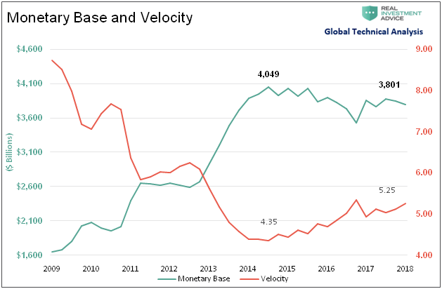
Data Courtesy: Federal Reserve
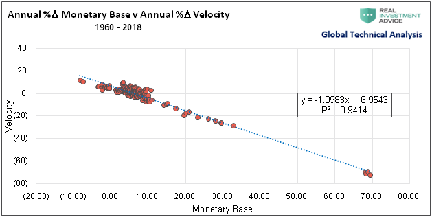
The scatter plot below highlights the near-perfect correlation (r-squared =0.9414) between %M and %V.
Data Courtesy: Federal Reserve
While %M and %V are highly correlated, it is important to grasp that the directional changes of %M and %V are not one for one. Note the formula on the graph that solves for %V given a level of %M is as follows:
%V = (-1.0983 * %M) + 6.9543
For instance, a 5% increase in %M would result in a change in velocity of 1.4628 [(-1.0983 * 5 )+6.9543 = 1.4628]. Without regard for output growth, the monetary components of the identity would produce a 6.4628%(5+1.4628) increase in prices. If we assume a 3% output-growth-rate, %P will equal 3.4628%.
The relationship between positive monetary growth and velocity is well known, as it has been the status-quo of inflation-forecasting for the better part of the last 60 years. Interestingly, however, the response of velocity (%V) is vastly different fora declining, as opposed to increasing, monetary base.Using quarterly observations beginning in 1960, the annual change in the monetary base (%M) has been negative in only 21 of 233 quarters (9%). Given the infrequency of money supply declines, do policymakers, economists, and market participants fully understand the ramifications of a sustained decrease in the monetary base?
The table below showing how velocity (%V) reacts to changes in %M, assuming constant output (%Q), helps us better understand the relationship between %M and %V.
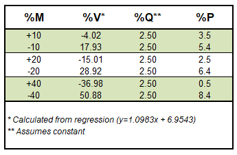
First, as demonstrated above, a reduction in the monetary base has a much larger magnitude-of-impact on velocity than an increase in the monetary base. Second, there exists what we call a positive “convexity” effect. At larger increments of percentage changes in the monetary base, the differential between the effects on %P widens. As shown, a 10% increase in %M, assuming a constant %Q, results in %P of 3.5%. However, a 10% decline in M results in a %P of 5.4%, almost 2% more despite an equal change in M. As shown, the“convexity” gap widens further when the money supply changes at greater rates.
Using the Federal Reserve’s guidance on the pace of QT, and assuming a constant %Q, we modeled the change in the monetary base (%M), the change in velocity (%V), and the resulting change in inflation (%P).
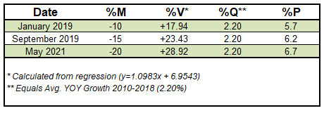
The forecast above is somewhat conservative as it is solely based on QT and doesn’t incorporateany further open market operations in the Fed’s quest to increase the Fed Funds rate.
This is where forming inflation expectations gets a little more complicated. If we assume the Fed follows through on their proposed actions, how much can economic growth offset increases in %P?When considering that important question, our primary concern, is that if economic growth weakens as a result of higher interest rates or other factors,the outlook is for higher inflation. In the example above, consider that by May of 2021 prices are expected to rise by 6.7% annually. Now recalculate that number for one percent (%Q) economic growth and %P increases further to 7.9%. On the other hand, assuming 4% economic growth would leave %P in May of 2021 around current levels of 2.7%.
Further Considerations
- Economic Growth (%Q)- Weaker growth is inflationary, while stronger growth reduces inflation. Will economic growth stumble with higher interest rates?Will tax cuts and fiscal stimulus keep growth humming along despite higher rates?
- Monetary Base (%M) – Close attention shouldbe paid to the Fed’s pace of QT. Further, we must also gauge the Fed’s intent to continue raising interest rates as this action also reduces %M.
- Velocity (%V) – Given the liquidity tightening actions the Fed is taking, and will likely continue to take, we should expect that the increase in %V has the potential to shock the markets, first bonds with equities close behind.
- Federal Reserve – How does their tightening posture change based on the factors above? Will they realize the pitfalls embodied in their policy and change course? Will they make a grave mistake by ramping up their inflation vigilance, not understanding that they are the ones stoking inflation’s embers?Alternatively, might it be possible the Fed is trying to thread the proverbial needle by carefully balancing economic growth with the monetary supply?
The last thing the Fed wants to do is generatehigher inflation with reduced economic growth, otherwise known as stagflation. As such, we must pay careful attention to Fed speeches and FOMC meeting minutes to glean a better understanding of how their policy expectations might change.
Stagflation, while historically rare, has proven to be an unfriendly investment climate for stocks and bonds. We think it is critical for investors to take their cues not only from Fed actions and talk, but also from economic growth outlooks and, maybe most important, changes in %V.
Summary
Assuming that further reductions in the money supply, higher velocity and weaker output ensues, we can confidently declare that inflationary pressures will increase. For investors, it is extremely important to be cognizant that such a conclusion runs counter to the popular narrative that slower growth and higher interest rates are deflationary. We do not want to take too much for granted in assuming the economists at the Fed are aware of these dynamics, but the potential for the Fed and investors to be caught by surprise while inflationary pressures rise is palpable. If the Fed were to be stoking inflation under a belief they are taming it, such an event would be a central banking error of historic proportions.
As emphasized above, it is essential to note that the size of their balance sheet is significantly larger than it ever has been. Therefore,sustained reductions in the balance sheet stand to be more significant than anything witnessed in the past. Given the Fed’s tone, alongside the identity and the factors discussed in this article, the potential for sharply increasing velocity is a distinct possibility. We venture that the equity and fixed income markets will not look favorably upon such an event,nor the increasing potential for stagflation.
Perhaps it is time to reconsider the Fed’s actions in this new light.
Michael Lebowitz, CFA is an Investment Analyst and Portfolio Manager for Clarity Financial, LLC specializing in macroeconomic research, valuations, asset allocation, and risk management. Michael has over 25 years of financial markets experience. In this time he has managed $50 billion+ institutional portfolios as well as sub $1 million individual portfolios. Michael is a partner at Real Investment Advice and RIA Pro Contributing Editor and Research Director. Co-founder of 720 Global. You can follow Michael on Twitter. This article is used here with permission and originally appeared here.

There are no comments to display.
Join the conversation
You can post now and register later. If you have an account, sign in now to post with your account.
Note: Your post will require moderator approval before it will be visible.