Leaderboard

Congrats on almost one year! @Djtux is a valuable member here and provides a great service which only continues to improve. Well worth it for SteadyOptions style trades. Not a paid endorsement, but I like to support good work .

It's almost the 1 year anniversary of the launch of the website. For anyone on the fence, i would encourage you to subscribe now to lock in the current price as i'm considering increasing it. I have some backend work to do on the payment system to be able to do that, but it's coming at some point. For existing subscribers, as long as you keep your subscription, nothing will change and thank you for the support.

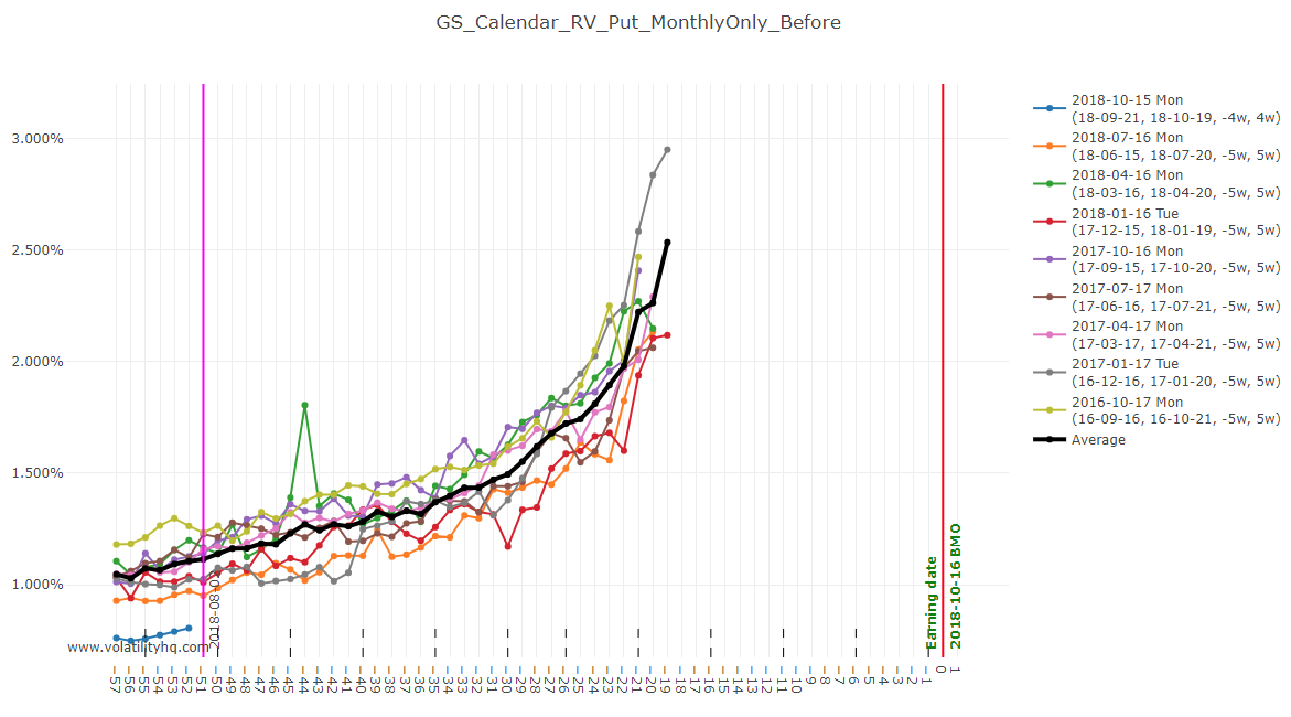
The main benefit of this chart is to show potential calendar spread gains over time - if the stock price stays near our strike. We KNOW that the front leg (expiring prior to earnings) is going to decline steadily which means the calendar RV chart will slope upward - so its not like our pre-earnings calendars where we compare RV, the important thing here is seeing the slope of the increase (unless, of course, something is way off from the average). That being the case, for the pre-pre-earnings analysis, its not a big deal if the monthly spreads have some 5 week and some 4 week calendars. I've been thinking about some general guideline for a trade like this: Open 6-8 weeks prior to short leg expiration. Look for stocks that show a tendency not to move too much between earnings periods (look at charts or do backtests). Look to close about 4 weeks prior to short expiration (no less than 3). From our hedged straddle experience we know that gamma can really accelerate on the short leg the closer you get to expiration so for a trade like this we want to be out before that happens - this is a bit counter-intuitive because the last 4 weeks is when the RV really starts to shoot upwards, but its also the timeframe where the spread becomes more sensitive to stock price movement and the profit tent narrows. Given these entry/exit timeframes use the pre-pre-earnings RV charts to show likely gain percentages if the stock price cooperates.

I'm with you on that!

Yes, I see them on Tradehawk

Those are good guidelines. I too, was looking to enter around the same time you mentioned, and exit well before heavy gamma kicks in. As far as underlying movement, we can look at the history of relative price move% to get some idea of how much tendency the underlying has moved in the past, during this specific time frame, to see if there are any repeating patterns, As far as the loss of value, on the short expiration, I think people tend to look in the wrong place for this. There is a big difference between the rate at which an option deteriorates, and the amount of premium an option loses. Most option sellers like to focus on the last 30 DTE, because time decay is the greatest. But, the gamma risk, associated with that is the highest. The thing that many people are missing, is that while an option may deteriorate at the fastest rate, during the last 30 DTE, it is not losing the most amount of it's value during that time. There is a period between 75 DTE- 50 DTE, ( it is hard to pinpoint the exact spot, but generally), where a 10 delta option will lose 50% of it's value, and not have much gamma risk associated with it that far away. An option is "born" with x amount of premium. By the the time it reaches T-30, it has already lost 90% of that premium. So, it is losing it's last 10% at the fastest rate of decline, with the most amount of gamma. So, this is sort of the worst spot to focus on for an option seller. Also, with regard to these 2 different calendar strategies, while a "normal" calendar, is a "long IV" position, one can make a case that a "pre earnings calendar" can be a short IV position. Look at the case where the long and short IV starts out at 45 and 43, and winds up at 95 and 50 IV....This does happen in some cases, and while the value of 1 vega is much greater, in the longer dated expiration, sometimes the front expiry IV gain is even greater than that. But, during non earnings times, a calendar is a long IV position. What is good about this trade is that the leg that you are long, is the first expiration post earnings. This is the expiry where, eventually most of the money will flow into, and will reach the highest IV of all expirations. This may not happen during the time frame of this trade, but the long leg will have a degree of "IV support".

I just added a new option on the Calendar RV page to support a 'pre-pre earnings' calendar. The short leg expires before the earnings date. That feature is in beta for now as i have not done extensive testing yet, and is slower than the rest of the functionalities because i have not implemented that much caching. Note that if you select the option to have the short leg before earnings, then you also need to select to use ONLY monthly options. Here is an example :

@NikTam Look at https://steadyoptions.com/forums/forum/topic/4666-discussion-gs-october-2018-trade/?do=findComment&comment=105877 for the start of the discussion of the 'pre-pre earnings' calendar. The short leg is the monthly expiry before earnings, not after earnings. @cuegis I'm working on that, i should have some prototype ready on the production website tonight. It won't be the fastest for now (page might load slower than the rest, there won't be caching like the rest of the website, but it's just to get something out there). Noted, i think it makes sense. Maybe i could show it in 2 spots : In the RV chart, when you hover a data point, i can show both the straddle/calendar price and the VIX I can also add a new chart to the Straddle RV page and the Calendar RV page. The new chart will be called VIX, and for each cycle i will show the VIX That way you can do a spot check on the VIX chart, and then drill down on the hover if needed. It's a start until we find a better way to represent that.